GTAP Models: A New Treatment for Investment
The dynamic GTAP Model uses a disequilibrium approach for modeling international capital mobility. A disequilibrium approach is necessary in order to reconcile the theory of investment with observed reality. Economic theory states that saving is allocated across regions to those investments with the highest rate of return. With perfect capital mobility, rates of return must be equalized across regions. In the dynamic GTAP Model, perfect capital mobility occurs only in the very long run. Investment is determined by the gradual movement of rates of return to equality across regions. This is the first use of the disequilibrium approach.A corollary of the capital mobility theory is that if rates of return in a particular country are very low, investment will fall and vice versa. Implementation of this theory however leads to a dilemma. In many cases actual investment, as reported in the national statistics, does not correspond to that predicted by this theory. That is, observed rates of return are low but investment is high. This was the case in Southeast Asia prior to the financial crisis. Such discrepancies can be rectified in one of two ways: firstly, the data can be altered so that theory and data are consistent; or alternatively, the theory can be modified to more accurately reflect the world. In the dynamic GTAP Model the latter method has been used. This has been achieved by incorporating errors in expectations about the actual rate of return. Thus investment is the result of the gradual movement of expected rates of return to equality across regions, but the expected rate of return may differ from the actual rate of return due to errors in expectations. This is the second use of the disequilibrium approach.
Determination of investment in the dynamic GTAP Model may be illustrated with the help of Figure 1, taken from Ianchovichina and McDougall (1999). The two curves in Figure 1 show the expected and actual rate of return schedules. The expected rate of return schedule depicts the relationship between the expected rate of return (rE) and capital stock (K), while the actual rate of return schedule shows the relationship between the actual rate of return (rA) and capital stock (K). These curves are downward sloping reflecting the belief that, as capital stocks increase, rates of return will fall, ceteris paribus. The difference between these two schedules represents the errors in expectations (i.e. the difference between observed data and the postulated theory). In any given year, there is a temporary equilibrium, global rate of return, rT, that ensures that global savings equal investment. This is depicted by the horizontal bar in Figure 1.
Investment in a particular year is determined by three mechanisms. The first is the desire to eliminate errors in expectations, which causes the expected rate of return to gradually move towards the actual rate of return. This involves the movement of the expected rate of return schedule towards the actual rate of return schedule (arrow 1 in Figure 1). In the case of China, the expected rate of return must rise to match the higher actual rates of return. Secondly gradual equalization across regions of rates of return requires the movement of the expected rate of return towards the temporary equilibrium (rT) (labeled 2 in Figure 1). With higher expected rates of return (as experienced in China) investment and capital stocks increase as the expected rate of return moves towards rT. The third mechanism converges the normal growth rate of capital stock over time towards a model-consistent value through the simulation. The normal growth rate of capital stock is the rate at which capital stock grows without affecting the rate of return. In the long-run equilibrium, actual (rA) and expected (rE) rates of return to capital in each region converge over time. The normal growth rate of the capital stock in each region also converges in the long-run equilibrium.
Figure 2 illustrates how actual and expected rates of return are driven to equality in the long run in the base case simulation. In China expected rates of return rise towards the actual rate of return (assuming no unexpected shocks). At the same time China's actual and expected rates of return gradually fall towards the long run equilibrium rate of return. Rates of return in Western Europe and the other countries also move towards this long run equilibrium.
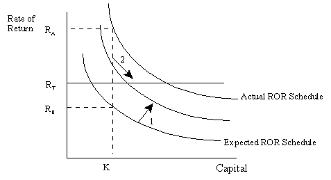
Figure 1: Expected and Actual Rate of Return Schedules. (Source: Adapted from Ianchovichina, McDougall and Hertel, 1999)
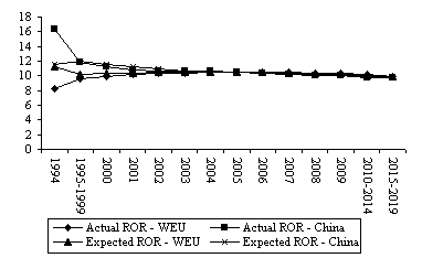
Figure 2: Base Case Actual and Expected Rates of Return. (Source: Walmsley and Hertel, 2000)
Last Modified: 4/3/2026 1:59:17 PM


